
About Me
Hola! I 'm Juan Pablo Triana Martinez, and I am a Biomedical AI Data Scientist 👋🏾.I focus on R&D development using Advanced Statistical Analysis, Digital Signal Processing, Multivariate Data Techniques, AI, ML, and Algorithms in IT or engineering domains.I am a driven researcher who implements many advanced data and engineering principles toolboxes 🧰 to help companies 💡Create Ideas💡, test them, and understand how feasible they are for creating them and bringing them to reality.
Skills Section

Python | SQL | Excel | PyTorch | TensorFlow | AWS RDS | AWS S3 | Matlab | Octave | Gitlab | Jira
Python Developer -> 3+ years
Cloud DevOps -> 2+ years
ML Frameworks -> 2+ years
Data Analytics -> 3+ years
Signal Processing -> 3+ years
R&D Projects -> 3+ years
Featured Projects
Deep Learning Binary Text Segmentation & PDF Semantic layout

Developed a binary text segmentation & PDF Semantic segmentation models, using the LinkNet-ResNet model, trained on DocLayNet 2023 dataset with COCO format.
Deep Learning Comparison
using MLOPs with AWS
Developed a MLOPs system, which compared a transformer, LSTM, and LSTM + attention model, to perform regression for oil and gold futures. All of this was deployed in AWS Sagemaker.
Multi-Agent Financial System
Using CrewAI
Developed, in a group project, a multi-agent financial analysis system of ticker-stocks, by integrating Python crewAI module framework, yfinance stock information, federal reserve, and OpenAI API.
Deep Learning Multi-Classification of MIDI -> Piano Rolls -> Composers using CNN vs CNN-LSTM approach
Developed a CNN vs CNN-LSTM system, transforming MIDI files into piano roll data, to perform multiclassification of different music composers.
Deep Learning Elderly Fall Detection/Prediction and Mitigation
Developed a Fall Detection system using the MultiCamFall dataset, leveraging 3D pose estimation and optical flow across multiple cameras.
FRAUD DETECTION IN CREDIT CARD HISTORY USING ML
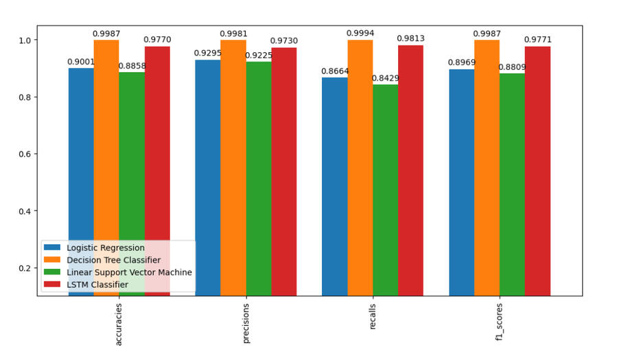
Developed a Credit Card Fraud Detection system as part of a group project. Implemented Logistic Regression, Linear Support Vector Machine, Decision Tree, and LSTM models
HOUSE PREDICTION USING OLS, LASSO, and GLM (log Link)
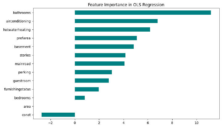
Developed a Credit House Prediction ML system in a group project. We applied OLS, Lasso, and GLM (log link) regression models in Python
SYNTHETHIC CHEST X-RAYS IMAGES USING VAEs and GAN
Used CNN encoders (VGG16, DenseNet) as building blocks to create different generative models (VAE, GMVAE, FSGMVAE, GAN) and assesed which approach created better synthethic chest X-rays Images.
Emotion Segmentation using Bi-directional LSTMS and BERT Embeddings
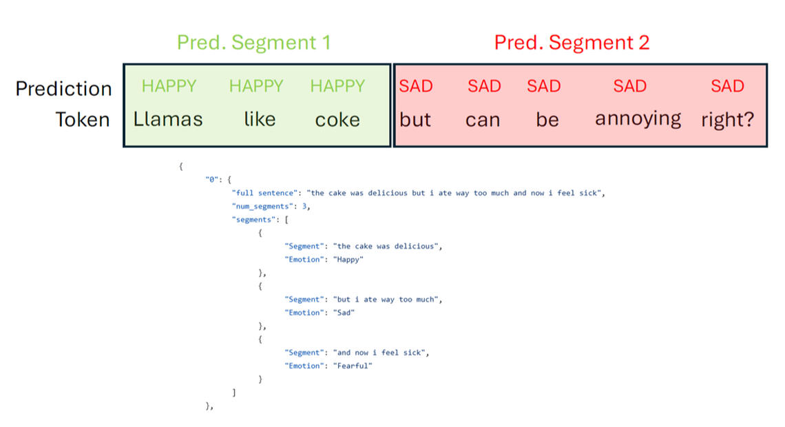
Using LLama-2 70B, and proper prompting, generated annotated emotion segmented phrases; which then were passed to a Bi-directional LSTM for emotion segmentation and classification.
GENERATE CHEST X-RAYS USING GMVAE AND DIFFERENT LOSSES (MSE AND BCE)
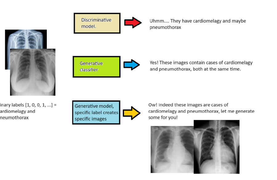
We took a look at the different kind of images generated from GMVAEs, by using different loss functions (MSE, BCE), and a positional embedding.
Professional Certifications
My list of academic, graduate, exam-based certifications.

Artificial Intelligence Graduate Certificate
June 2024
Online E-learning Certificates
My list of Online, E-learning, Most relevant online certificates.

Specialized Program - Machine Learning
May 2024

SQL For Data Science
February 2023

Using Databases with Python
February 2023
Deep Learning Binary Text Segmentation & PDF Semantic layout using LinkNet-ResNet -> Chestnut
using PyTorch in Python.
Project Links below

The rapid and reliable digitalization of physical documents into structured electronic formats has become a critical need across modern industries. Organizations increasingly depend on transforming sensitive, paper-based records into secure, searchable digital databases to improve accessibility, efficiency, and data-driven decision-making. In this report, we showcase how a LinkNet-ResNet model, ChestNut, was implemented on the DocLayNet Dataset (Pfitzmann, B, et al. 2023).
results? the following are divided into binary segmentation and PDF semantic segmentation results:
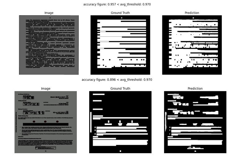
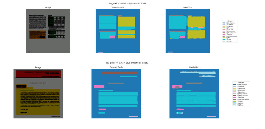
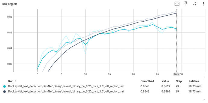
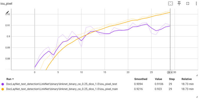
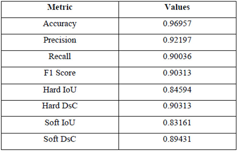
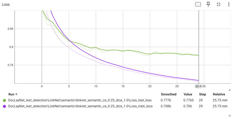
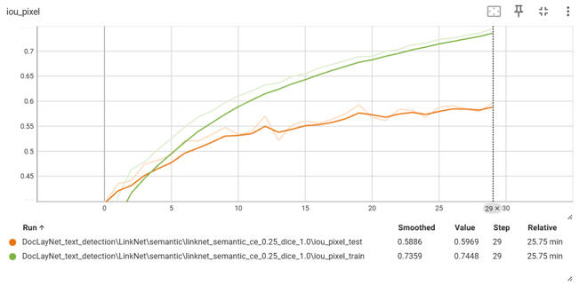
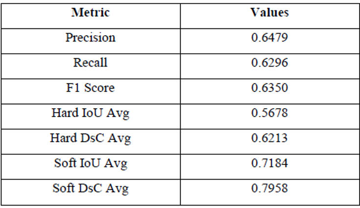
This small model of 11 million parameters can achieve production-level metrics for binary text segmentation masks (Soft IoU: 0.83, Soft DsC: 0.89, F1 Score: 0.90) and foundational metrics for research in PDF semantic segmentation (Soft IoU: 0.72, Soft DsC: 0.80, F1 Score: 0.64).
Binary Text Graphs and Results
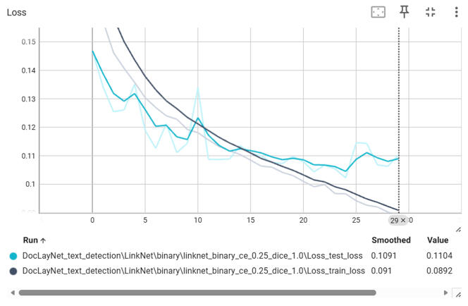
The following are the graphs related to the training loss function, the Intersection over union and Dice coefficient (i.e., ignoring background pixels), and ML metrics.
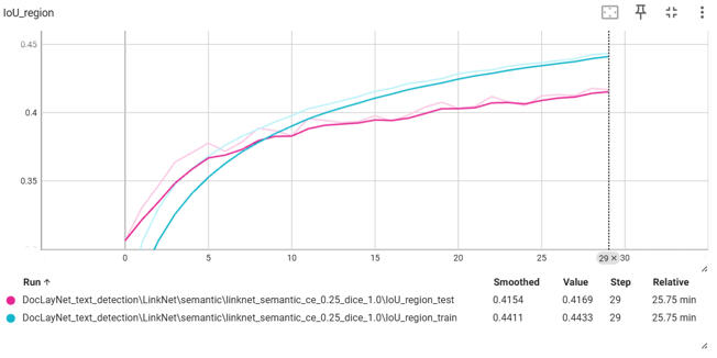
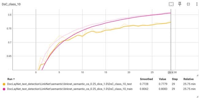
PDF Semantic Graphs and Results
The following are the graphs related to the training loss function, the Intersection over union and Dice coefficient (i.e., ignoring background pixels), and ML metrics for the semantic case.Here, class 10 refers to the text. Although the results were not production-level, the research metrics show an IoU of around 0.7~0.8. This is a good research starting phase for further improvements.
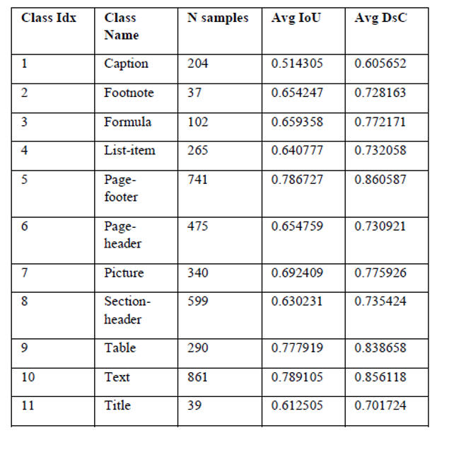
ConclusionDual-task evaluation: Assessed a compact LinkNet–ResNet (~11M parameters) for both binary text segmentation and semantic PDF segmentation on limited GPU resources.Strong binary segmentation performance: Achieved 96.95% accuracy, >90% precision/recall, and 0.90 Dice score, producing reliable text masks suitable for OCR pipelines.Efficient architecture:Demonstrated that a lightweight model can deliver high-quality results while remaining feasible for smaller GPUs and scalable applications.Promising semantic learning: Despite lower hard metrics, soft IoU (0.7–0.8) indicates the model successfully learns meaningful class probability distributions.Clear path for improvement: Future work includes expanding datasets, adding regularization (dropout, augmentation), exploring attention/multi-scale architectures, and optimizing for real-world deployment
Deep Learning Comparison
to predict oil and gold futures
using MLOPs with AWS
Project Links below
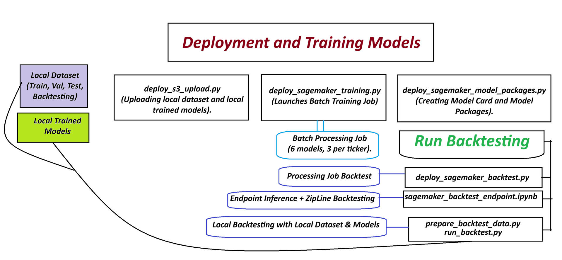
Machine Learning Operations explains the system design requirements and steps to train, deploy, and test an AI/ML model in testing and production environments, ready for multiple shadow-container testing or real-world use. That being said, alongside this graduate-level course, we implemented a comprehensive MLOPs system using AWS services (i.e., AWS Sagemaker, AWS S3, AWS Batch training, AWS Batch and Endpoint Inference, AWS CloudWatch Metrics, CI/CD, etc.). Our Final group project consisted of implementing an MLOps Batch training system of deep learning regression models, specifically an LSTM model, a bidirectional LSTM model with attention, and a transformer encoder-based architecture to determine which was the best in performing regression for gold futures (i.e, Ticker CG=F) and oil futures (i.e, Ticker CL = F).
Results? The results were interesting. By using the ZipLine Python module for backtesting in a production environment dataset (i.e, from 2019 to 2026), of python trading algorithm, we created an algorithm based on 70% Model vote, 15% EMA (i.e, exponential moving average), 15% McClellan Oscillator by sending buy/sell shares per signal, the total return of the portfolio using the three deep learning models was of 4.12%, with 0.1758 sharpe ratio, and Max drawdown of 60.35%.
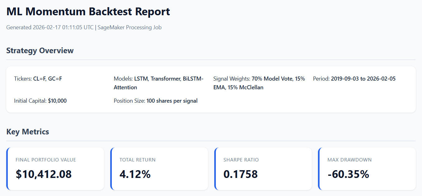
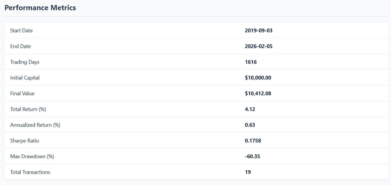
Although the results were not great, looking closer into each deep learning model's accuracy regression metrics (i.e, RMSE, MSE, MAE, and MAPE%), the LSTM and BiLSTM_Attention had much better regression metrics in validation and test splits on gold and oil futures vs the transformer models.
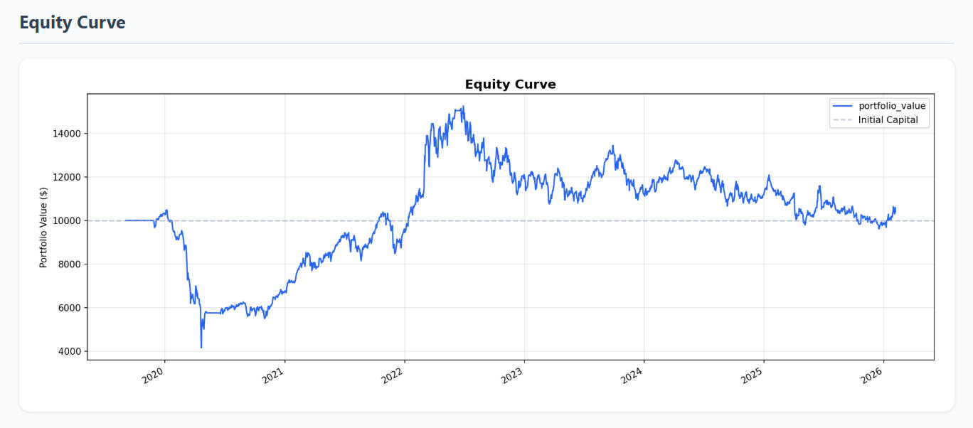
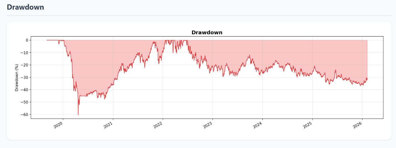
Additionally, looking into the backtesting equity curve, there was a maximum value of 14500 USD of portfolio value at 2022, suggesting that CI/CD fine-tuning could have prevented the losses from 2022 to 2026. Although a research moment, this gives us insights about how to deploy regression models with trading strategies using MLOPs steps.
Key Project Structure
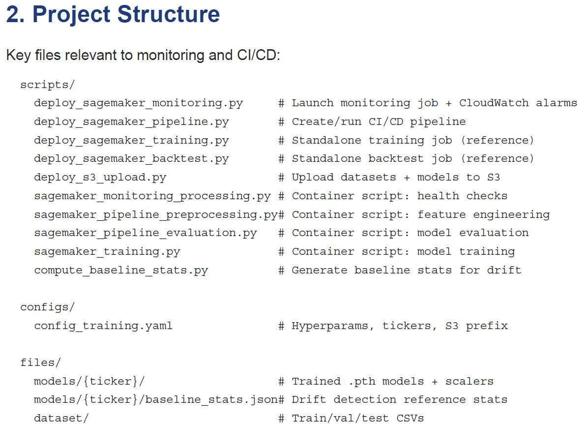
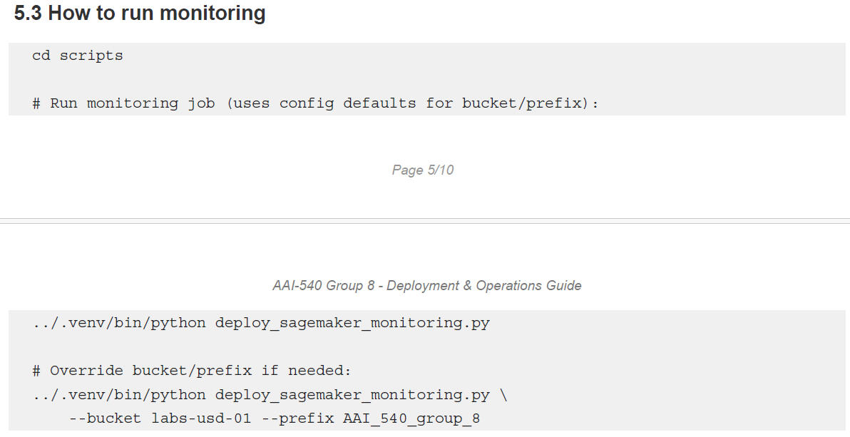
This entire project requires AWS Credentials in order to run in AWS Sagemaker, but the general steps are the following once that's settled:
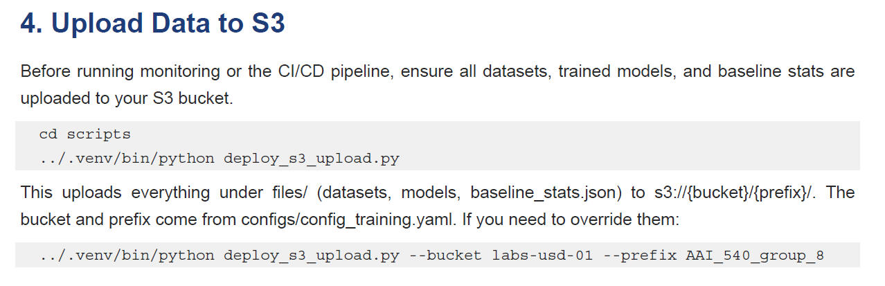
Deploy Monitoring SystemData Drift Detection (Kolmogorov-Smirnov Test)
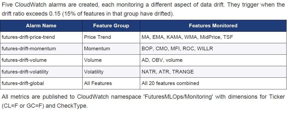
Compares the distribution of each of the 20 features in production data against the training baseline. Uses the two-sample KS test: if the p-value is below 0.05, that feature has drifted. Features are grouped into four buckets (price_trend, momentum, volume, volatility) and the drift ratio per bucket is reported as a CloudWatch metric.Structural Break Detection (CUSUM)
Applies the Cumulative Sum (CUSUM) algorithm to the close price series. If the cumulative deviation from the mean exceeds a threshold, it signals a structural break (e.g. a regime change in the market). A structural break means the statistical properties of the price series have fundamentally changed, which may invalidate model assumptions.Model Disagreement Score
indicates that models (LSTM, Transformer, BiLSTM-Attention) generate predictions on the same production data. The coefficient of variation (std / mean) across the three predictions is computed. High disagreement (>0.10) ndicates the models are uncertain or seeing data outside their training distribution.Prediction Anomaly Detection
Each model's mean prediction is compared against the training baseline (mean +/- 2 standard deviations). If a prediction falls outside this range, it's flagged as anomalous. This catches cases where a model produces
unrealistic forecasts.How to read the metrics?drift_ratios:
fraction of features drifted per bucket (0.0 = no drift, 1.0 = all drifted).structural_break:
true/false, whether a regime change was detected.model_disagreement:
coefficient of variation across models (lower is better).prediction_anomalies:
which models produced out-of-range predictions.

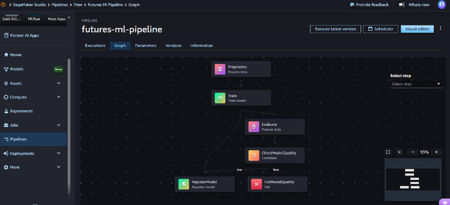
Deploy CI/CDStep 1: Preprocess
A Processing Job that: installs TA-Lib, loads raw OHLCV data from S3, computes the 20 technical indicator features (same as local training), and splits the data into train (60%), validation (20%), and test (20%) sets. Data is saved UNSCALED - the training step handles scaling.Step 2: Train
A Training Job using the sagemaker_training.py entry point (same script as standalone training). Trains the specified model (default: LSTM) on the specified ticker (default: CL=F) for N epochs (default: 5 for validation,
200 for production). Outputs the trained model .pth file, scalers, and metadata as model.tar.gz.Step 3: Evaluate
A Processing Job that loads the trained model and scalers from Step 2, scales the test data from Step 1, runs inference, and computes regression metrics: MSE, RMSE, MAE. Writes evaluation.json for the quality gate.Step 4: CheckModelQuality (Condition)
A quality gate that reads the MSE from evaluation.json. If MSE <= threshold (default: 0.05 for validation, 0.005 for production), the model passes and proceeds to registration. Otherwise, the pipeline fails.Step 5a: RegisterModel (if passed)
Registers the trained model in the SageMaker Model Registry under the appropriate package group (futures-cl-models for CL=F, futures-gc-models for GC=F) with status 'PendingManualApproval'. This creates a versioned record of the model for governance and deployment tracking.Step 5b: FailModelQuality (if failed)
If MSE exceeds the threshold, the pipeline ends with an explicit failure message indicating the model did not meet quality standards.
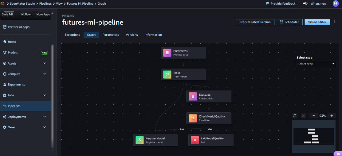
Futures ML Pipeline: With the final AWS Sagemaker Pipeline, my group and I have implemented a full MLOPs system that allows us to compare between LSTMs, Transformers, and LSTMs+ attention mechanism layers models for regression problems with gold and oil futures.Thank you so much for looking into this project! If you want to know how this entire MLOPs pipeline works in AWS, feel free to click below the Github links containing all of the codes in boto3 with Python
AAI-540: Specific Github Project Links to understand code🖥️
- Python Code Sagemaker Monitoring
- Python Code Sagemaker Pipeline
- Python Code Sagemaker Training
- Python Code Sagemaker backtest
- Python Deploy s3 and upload models and datasets
- Container script: health checks
- Container script: feature engineering
- Container Script: Model Evaluation
- Container Script: Model Training
- Python Code: Baseline stats for drift
Multi-Agent Financial System
Using CrewAI
Project Links below
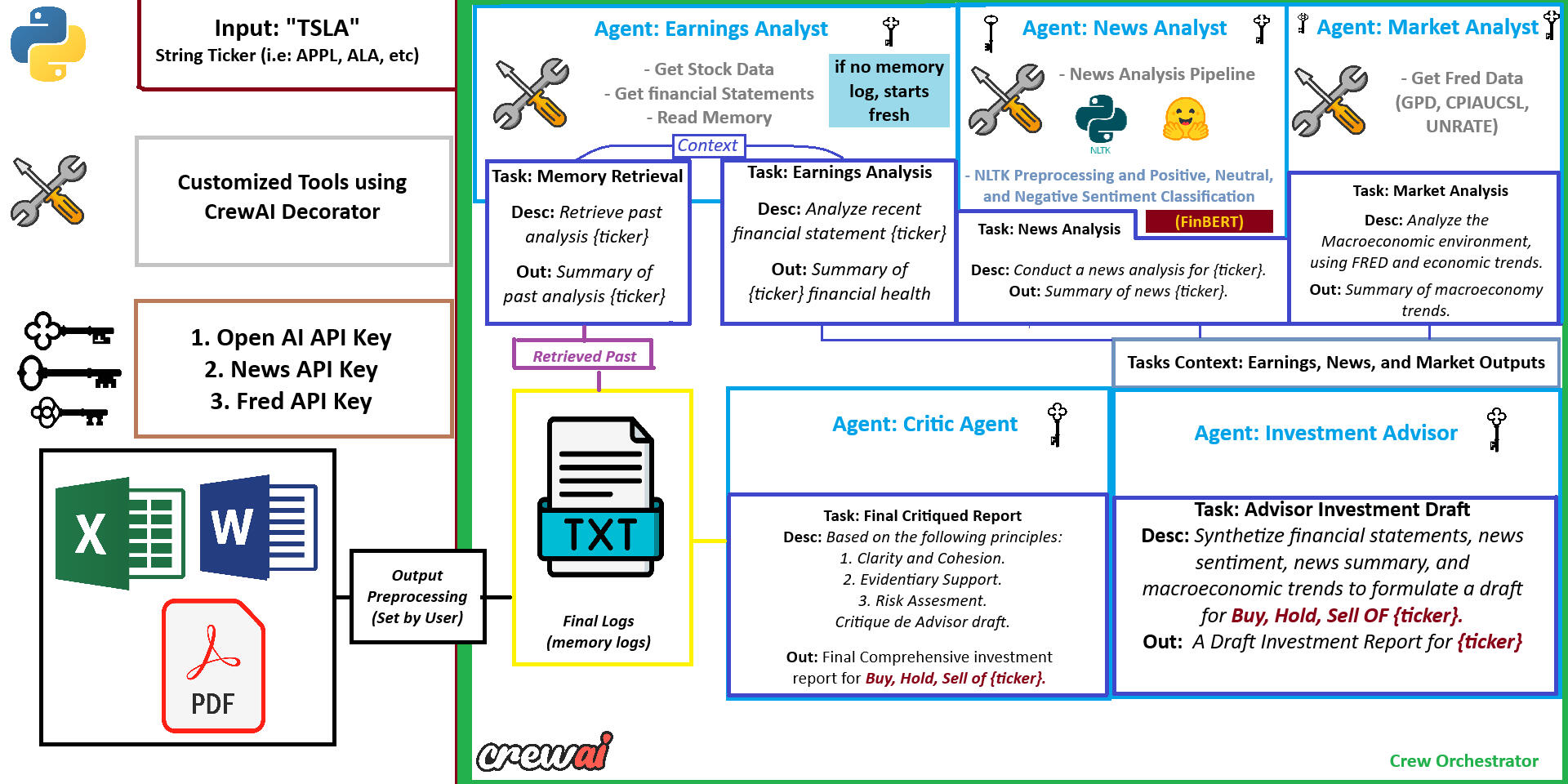
Why this Project? In 2025, one of the clear advancements of generative AI in the NLP domain has been the adoption of LLMs to create agentic AIs. Strangely enough, this coincided with the development of much more powerful GPUs and TPUs by big tech corporations as well. With that being said, the need to understand how to fine-tune, orchestrate, and chain different LLMs agents inputs-outputs to analyze, reason, and create a desired data output is now possible. In this final project for the MSAAI program at USD, my group and I developed a multi-financial agent analysis (earnings, news, and market analysts, investment advisor, and Critic agent) to generate financial reports of specific stock.
Results? The results of this 5-multi agent financial system is the generation of a concise, readable, and comprehensible financial report of a desired stock
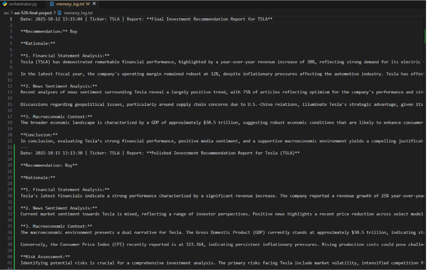
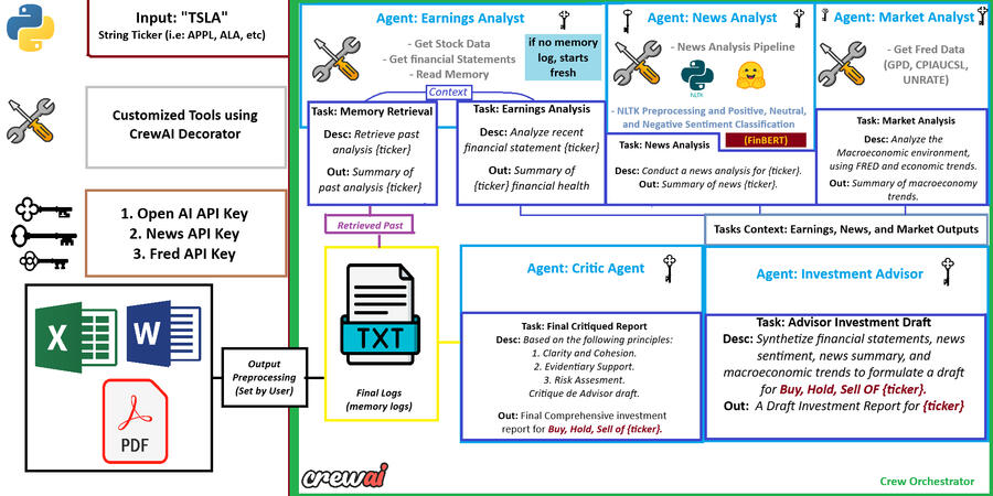
As shown in the image below, the report is saved in a log.txt file which contains a specific structure of a financial statement analysis, news statement analysis, and a macroeconomic environment pertinent to the company. How is this even possible?
Earnings Analyst Agent
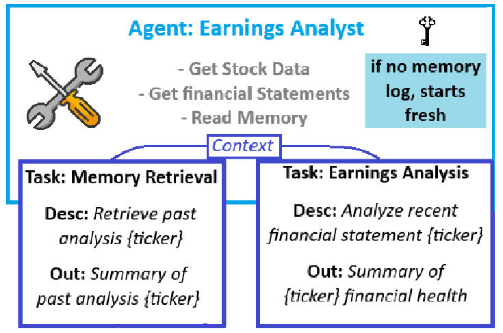
Earnings Analyst Agent: The first block of the information diagram is to create the earnings analyst agent. This agent, built with OpenAI API Key, uses customized Crewai tools to get stock data, get the corresponding financial statements, and read from memory IF there were past analyses found in the log file. This ensures the first step of the financial analysis, retrieving the relevant financial information from current and past.
News Analyst Agent
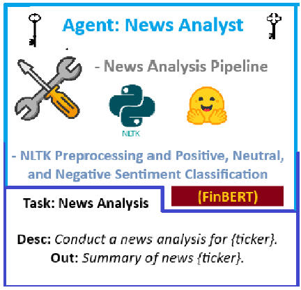
News Analyst Agent: The second block is the news analyst agent. Here, the news analysis pipeline contains python nltk text preprocessing steps to pre-process the retrieved text in a proper format. Followed by this, using the huggingface transformer model FinBERT, a sentiment classification of the company's news is performed as well (Positive, Negative, and Neutral). The output of this is the second source of information, a news summary report of the company's behaviour in the market, and what's the market sentiment towards it.
Market Analyst Agent
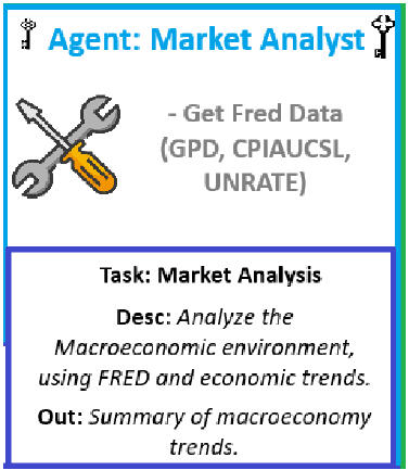
Market Analyst Agent: The following is called the market analyst agent. This one uses the Federal Reserve of St. Louis API key information to retrieve macroeconomic trends (GDP, CPIAUCSL, UNRATE) to create a summary of the trends. This is the last required summary to pass for the investment advisor.
Investment Analyst Agent
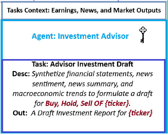
Investment Advisor: Using the earnings, market, and news analyst summary outputs; these are used as Context for the investment analyst agent to generate a Draft of an investment report! This would be further passed to a financial critic agent to polish it and present it!
Financial Critic Agent
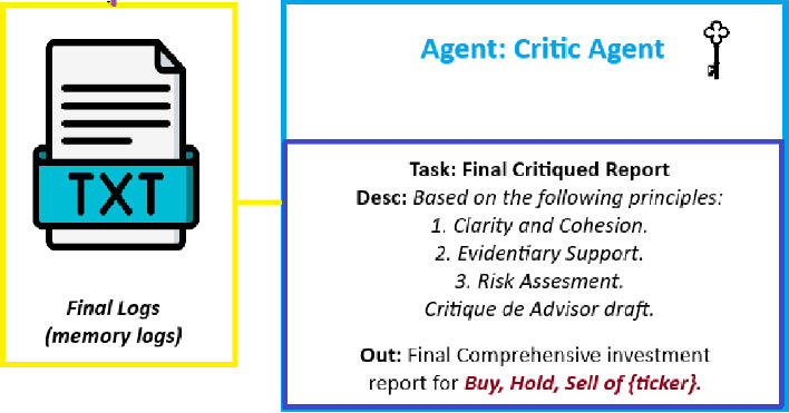
Financial Critic Agent: With the final agent, this critic agent would create the final report and output it to the final.text memory logs. Having the specific format mentioned in the very beginning.Thank you so much for looking into this project! If you want to know how these agents work, feel free to click below the Github links containing all of the codes in CrewAI.
AAI-520: Specific Github Project Links to understand code🖥️
- Crewai Earnings Analyst Agent
- Crewai News Analyst Agent
- Crewai Market Analyst Agent
- Crewai Investment Advisor Agent
- Crewai Financial Advisor Critic Agent
- Crewai Earnings Analyst Financial tools (Stock data and Financial Statements)
- Crewai Earnings Analyst memory log file tools
- Crewai Market Analyst tool (Federal Reserve)
- Crewai News Analyst Customized tools (NewsAPI and FINBERT Sentiment Classification)
Deep Learning Multi-Classification of MIDI -> Piano Rolls -> Composers using CNN vs CNN-LSTM approach
Project Links below
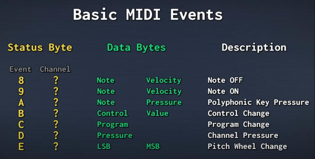
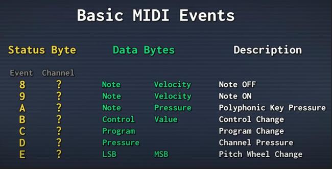
Why this Project? Machine Learning and Deep Learning capabilities are not only limited to structured, discrete data, but also to unstructured, continuous data. As one of the final projects for my graduate course in my Master of Science in AI from the University of San Diego, my group and I had to create a deep learning solution to classify 4 different composers (Bach, Beethoven, Chopin, Mozart) from MIDI files.As the image above shows, MIDI files are music “cooking instructions” used in analog-to-digital devices, converting music into digital audio files for the machine to understand.
Results: The following contains the CNN Confusion Matrix and ML metrics vs CNN-LSTM confusion matrix and ML metrics.
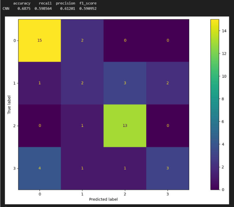
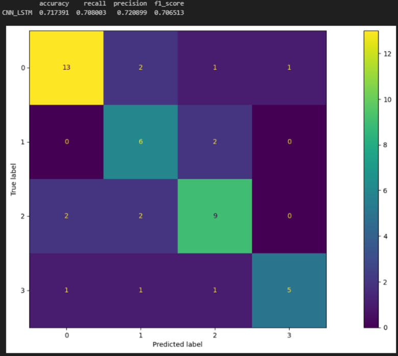
As evidenced by the results, CNN-LSTM performs significantly better than the CNN model for multiclassification, there are key things to consider for future analyses, and these are:• Addressing Train/Val/Test Splits imbalances: Truly, although the splits were done in detail, this project didn’t address the issue of differences of probability distributions, which it means that some results can be skewed or not truthful to the true distribution of data.• GPU training: Previous tests with GPU showed it’s possible to push the CNN-LSTM model to 81% average across all metrics. Nevertheless, it’s imperative that, depending on the computing resources available (i.e. No GPU available), choosing between training a CNN-LSTM model more than 75% can become a matter of hours or days.• Possible Data Leakage: There is the possibility of data leakage when transferring downloaded files from internet using customized classes to extract only the desired 4 composers. BE CAUTIOUS. Althought the behaviour of splits is the same across different computers, it appears that some copies of data leaked across (the University found that error). Please, this is more of an educational project to illustrate skills in deep learning, not to be used in production environments.
Data Pre-processing: MIDI file Metadata -> CNN Piano rolls -> Equalized Piano Rolls:There are indeed a couple of MIDI files' metadata that we are going to use to create our 2D piano roll:• set_tempo: In MIDI, tempo refers to the period in μs (microseconds)/beat.
Normally, we deal with the following:
• 500,000 or 0.5 s/beat. Which means an event frequency of 2 Hz
• 1,000,000 or 1 s/beat. Which means an event frequency of 1 Hz
Using the Nyquist-Shannon Sampling Theorem, we converted MIDI files to piano rolls based on symbolic representation using event frequency. This means we need a minimum fs around 4 or 2 Hz to represent Changes of events, NOT pitch frequency, which is what we want.To settle things, we would use fs = 10. Now what is fs? This is a frequency sample. Let's do an example:• Suppose we have a track of a total of 250 seconds.
• With an fs = 10, the discretized tensor would have an axis of 2500.
• And so on, so on.
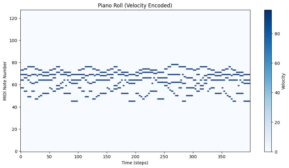
NOW, what we want to capture is a 3D tensor that would be the following per MIDI file:- (128 * Discretized time): These contain the following:a. First Axis: All 128 possible Octave pitch notes, values with pitch range note value from 0 to 127.
b. Second Axis: Time the track took, values with ranges from 0 to fs * time.
c. Values first Axis: torch.tensor[pitch, t] = velocity, at each time step, we would assign for the specific pitch axis, the value of velocity
Time here! How do we define it, with the following formula (tempo is in milliseconds, so we need to divide it by 1,000,000 to make it seconds):

Lastly, the last step to do is to equalize each piano roll to a certain discrete length across all. This is imperative to ensure model data is consistent and can be used in a deep learning pipeline for training.To do this, the analysis was done to estimate the proper value based on the histogram distribution of the discretized song lengths.
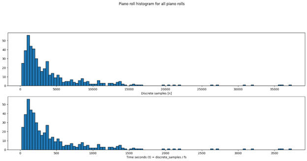
The observations of the lengths of different time songs show that it’s skewed to the left, meaning that we would like to select a right size like this:• If the song has more than the median of lengths, then truncate the song up to the median.
• If the song has less than the median of lengths, then tile or repeat the song up to the median.With these rules, we were able to obtain tensors of size (N, H, W) where:• N was equal to the total number of songs available across all 4 composers
• H was the height of the octave ranges, 128 to be precise
• Width was the discretized equalized length of the songs, with a median is 2515.
This data is key to pointing out that technically it is (N, C, H ,W). Where C is equal to 1 since the piano roll acts like a 1-channel image.Why is this important? With some PyTorch Tensors manipulation, combined with a PyTorch Data Loader and PyTorch Dataset, we were able to retrieve (B, 1, 128, 2515), where B refers to the Batch size used for CNN model training. For the CNN-LSTM model, we had to add dimension called sequence, which results in tensors of size (B, S, 1, 128, 2515).
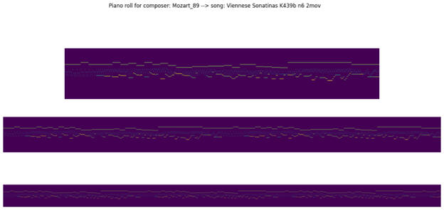
Project Steps1. Data Downloading/Preparation: All data from MIDI files was downloaded, and further separated into subfolders to analyze only four desired composers: Bach, Beethoven, Chopin, and Mozart.2. Data Cleaning/Preparation: Since the CNN and CNN-LSTM models required 2D data, the MIDI files were preprocessed using customized classes, contained in src/, in order to obtain from music.midi -> np.ndarray of piano rolls.3. EDA Piano Roll Data: Once the piano rolls were found, EDA was done to see how the piano rolls of different durations behaved. Using different discretized times of songs, we found the median of all songs and used it as a threshold to Equalize all songs.4. CNN Model Training and Analysis: The models were evaluated based on models were evaluated based on F1 score, accuracy, precision, recall, and F1 Scores. We also used visualized confusion matrices
5. CNN-LSTM Model Training and Analysis. Same as CNN, but with the added caveat of a sequence length used.
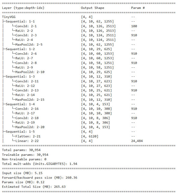
Model ArchitecturesThe following contains a torchinfo summary of the CNN model with the following hyperparameters:, Batch size = 4, Channel in = 1, Height = 128, Width = 2515
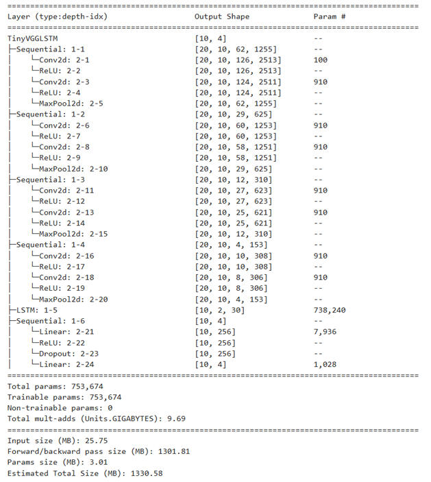
The following contains a torchinfo summary of the CNN-LSTM model with the following hyperparameters:, Batch size = 10,
Sequence Length = 2, Channel in = 1, Height = 128, Width = 2515
If you want to learn more about the project, below are the links to the specific code sections that break the code, step by step.🖱️
AAI-511: Specific Github Project Links to understand code🖥️
- Data Download Jupyter Notebook
- Data Exploration EDA Analysis Jupyter Notebook
- Data Piano Roll Extraction Jupyter Notebook
- Data Piano Roll extraction using Python Package
- CNN Baseline Jupyter Notebook
- CNN-LSTM Jupyter Notebook
Deep Learning Elderly Fall Detection/Prediction and Mitigation
Project Links below
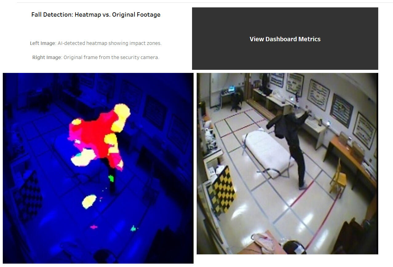
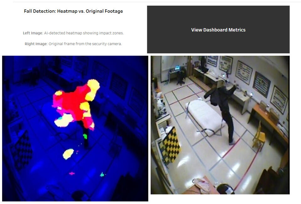
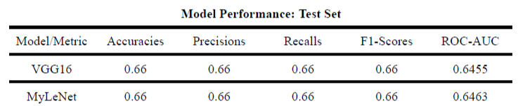
Why This Project?: Falls among older adults are a major public health concern, yet much of the AI research in this area has been focused on a binary classification problem—detecting whether a fall has already occurred. However, true innovation lies in the ability to predict falls before they happen.In this project, we explored how current deep learning approaches, particularly Convolutional Neural Networks (CNNs), classify falls using optical flow gradients to capture motion. We then used a VGG16 fine-tuned to our task, and a customized/optimizer MyLeNet, to see how these approaches perform for fall detection (not fall prediction).To push the boundaries of fall prediction, we proposed a CNN-LSTM system that integrates temporal dynamics for enhanced forecasting. Our approach involves: 3D Pose Estimation – Extracting movement information from each frame, Predictive Horizon of 600 ms – The first 500 ms capture pre-fall motion, while the next 100 ms include an overlapping window containing fall event.Results: Our CNN-LSTM system outperformed standard CNN models—not only in fall detection accuracy but also in fall prediction capabilities. A key focus of our work was recall, ensuring that false negatives (instances where a fall occurs but is not detected) were minimized, as they pose a critical risk. The following results compare the CNN-LSTM approach with CNN-based models, highlighting the improvements in both precision and predictive reliability.

Dataset The dataset we used was the multiple camera fall dataset created from Auvinet, et al. from the University of Montreal in 2010. Using this dataset, our intention is, by using all the data from the 8 different angles with 23-24 different scenarios than involve falling, as well as normal human activities, to be able to predict a fall from a single camera.
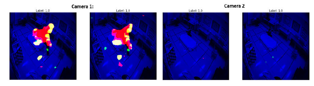
Data Preprocessing: CNN approachesTo emulate the current research on fall prediction; we followed what the literature suggests about capturing motion among frames. In specific conditions; where the movement is not erratic, there is no change in illumination, and there is no occlusion, a camera can approximate the flow of motion by using optical flow gradients. We used the Flow Farnerback algorithm in built in CV2 submodule in python, with the following parameters:

How were the optical flow gradients? well.... it appears that for cameras where the user is really far away a certain distance, the algorithm is unable to capture that optical flow motion. Which indeed has affected the dataset passed to the CNNs in order to classify fall/no fall.
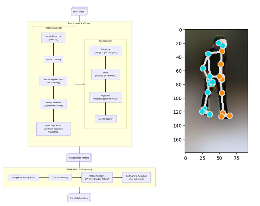
Data Preprocessing: CNN-LSTMFor the CNN-LSTM Approach, it was quite radically different how motion was captured. The main idea was to pass it to a 3D Mode estimation model (yolo11), retrieve the joints information of the person while moving, and use this as frames to a CNN-LSTM with predictive horizon, to predict a fall.
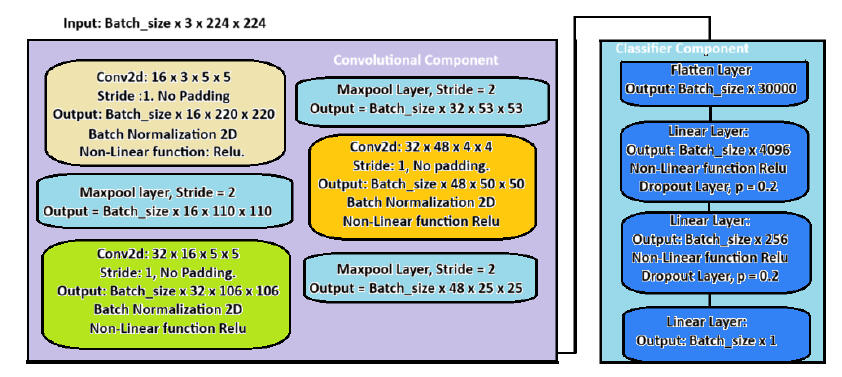
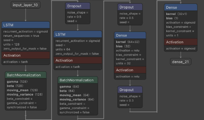
Model Architectures The following contain the model architectures used for the MyLeNet, and the CNN-LSTM model. We didn't add the VGG16 per see, since the fine-tuning meant we only change the last classifier layer to match the number of classes we have for a binary fall prediction task.
If you want to learn more about the project, below are the links to the specific code sections that break the code, step by step.🖱️
AAI-530: Specific Github Project Links to understand code🖥️
CNN-LSTM Codes
CNN Codes
- Project Code link: Data preprocessing, CNN Optical flow gradient download in .npy format
- Project Code link: Utils, dataset for single image frame reading
- Project Code link: Utils, dataset for series of frame images, series reading.
- Project Code link: Customized MyLeNet CNN
- Project Code link: VGG16 CNN finetuned
FRAUD DETECTION IN CREDIT CARD HISTORY USING ML
Project Links below
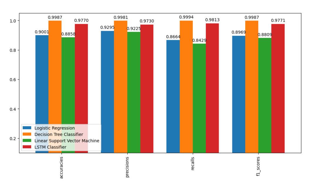
Why this project? With the advancement of Machine Learning and Deep Learning, one of the applications in which many of these systems were implemented to classify fraudulent transactions in the banking sector. This project contains a step-by-step recipe that encodes non-numerical high ordinal features (transaction datetime, date of birth, zip code) and low binary ordinal features (gender, status). This was followed up by standardization and oversampling of the unbalanced datasets using SMOTE techniques. Finally, we tested different ML algorithms, as well as a LSTM neural network In this task.
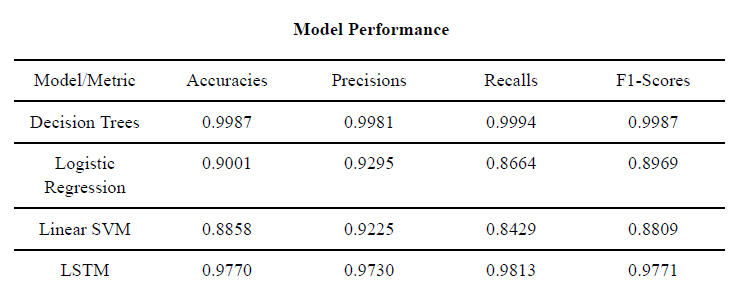
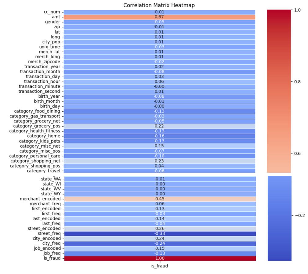
Results: We were surprised by the results we obtained for Decision Trees on our dataset, as they showed exceptionally high accuracy (F1 scores: Decision Trees = 0.9988; Logistic Regression =0.8969; Linear SVMs = 0.8809; Long Short Term Memory (LSTM) = 0.9771 ) . This even led us to question our initial research. However, upon closer examination, we realized that expanding our original feature set from 20 to 96 numerical features may have significantly contributed to these outstanding results.The following tables present the performance of various machine learning algorithms tested, along with the results for the LSTM model.

Dataset and PreprocessingWe had an intial dataset of credit card history transactions from 2019-2020, of 1296675 entroes of 22 features each entry. Our target variables is a binary variables of fraudenelt/non-feaudulkent transaction. Due to the presence of many non-numerical features, we did the following preprocessing:
Drop Unique Identifiers from credit card history Unnamed:0, trans_num.
Fill Nan values in merch_zipcode with the median value.
Obtain the datetime features from the transaction and the date of birth datetimes.
Obtain low categorical features, binary and small unique identifiers: gender, category, state
Obtain high categorical features, using frequency and target encoding: merchant, first, last, street, city, job
Handle balanced dataset: Lastly, we use SMOTE to handle the inbalanced dataset between fraudulent/non-fraudulent transactions.
If you want to learn more about the project, below are the links to the specific code sections that break the code, step by step.🖱️
AAI-501: Specific Github Project Links to understand code🖥️
- Project Code link: Dataset Link | Credit Card History
- Project Code link: Utils, Downloads the data from Kaggle.
- Project Code link: utils, Preprocess the features to numerical and more detailed features.
- Project Code Link: Jupyter notebook for feature encoding and extraction.
- Project Code link: All different ML models
HOUSE PREDICTION USING OLS, LASSO, and GLM (log Link)
Project Links below
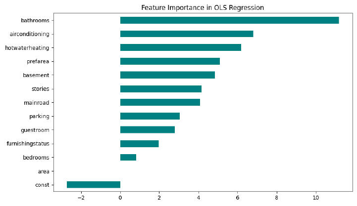
Why this project? Across my academic path in AI and ML. I have done projects that involved using many of the complex architectures used on the forefront. Nevertheless, I have disregarded the power as well of how we can setup problems and use much simpler ML models to solve problems. I had the opportunity to do this in the beginning of my Master's in AI. This project aims to use regression models for OLS, Lasso, and GLM (link = log).
Results We used metrics of Train-R-squared, Test-R-squared, and RMSE, to measure the model that was the best fit. Additionally, we conducted two tests: one using all features after pre-processing, and another using only highly correlated features. The results, at the beginning, the GLM (log) link performed better in the train data; when it came to the test data, the OLS was the best one, followed by the Lasso regression.
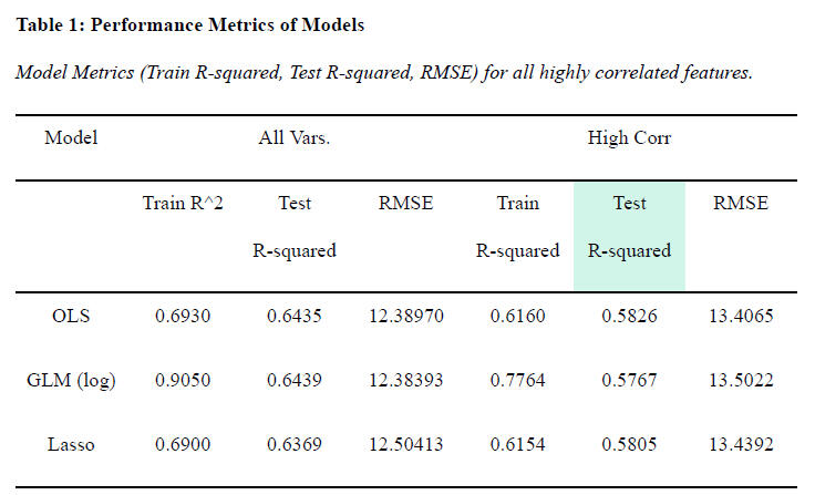
Data Preprocessing and Heatmap EDA Analysis
The first step we had to do was to preprocess the data in order to have only proper numerical features against our target variable (price). For this we did:
Remove Missing Data
Encoded Categorical Variables
Feature Standardization Scaling
Normalization of target variable
Following this, we performed a correlation matrix in order to see the feature relationships. We took the first row of this matrix, and selected two different datasets: One containing all features, and one containing only High correlation features (greater than 0.4).
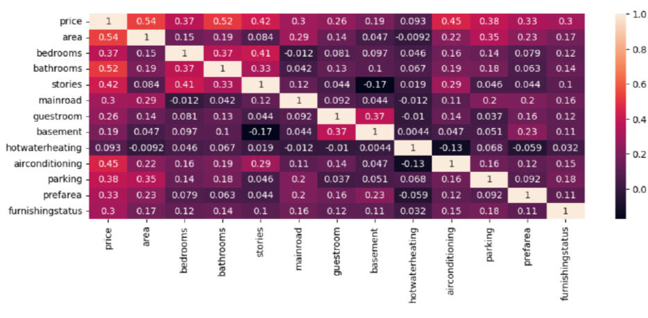
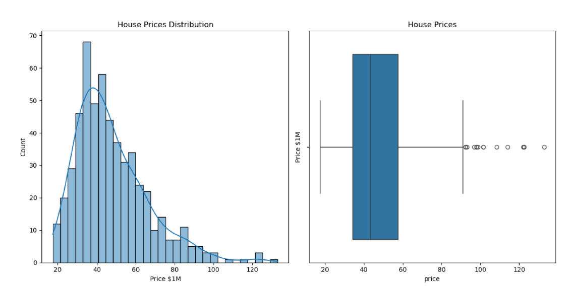
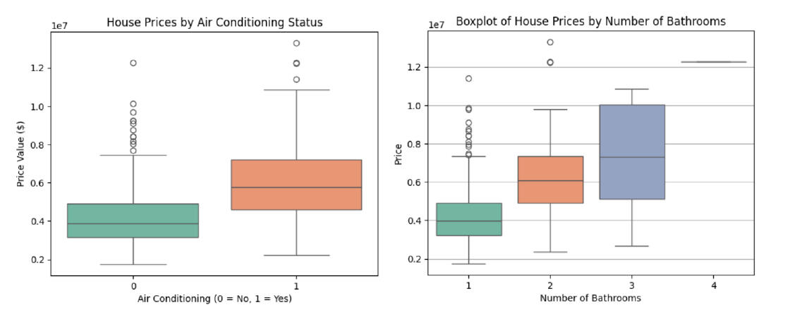
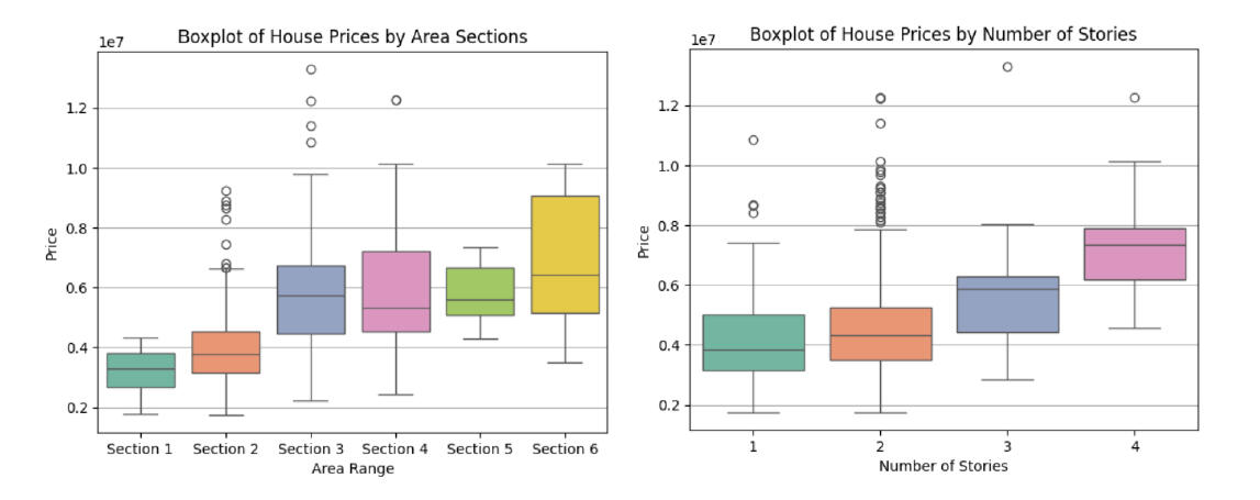
With this information, the next step was to analyze the distribution of the target variable (house price) and examine the relationships between highly correlated features and price. We found that the price distribution was skewed to the left, which led us to test whether a Generalized Linear Model (GLM) with a log transformation could better capture this relationship. Additionally, boxplots revealed how specific features significantly influenced price increases.
If you want to learn more about the project, below are the links to the specific code sections that break the code, step by step.🖱️
AAI-500: Specific Github Project Links to understand code🖥️
SYNTHETHIC CHEST X-RAYS IMAGES USING VAEs and GAN
Project Links below
Date: June 3rd, 2024
Group Members:
Abhishek Kumar
Juan Pablo Triana Martinez
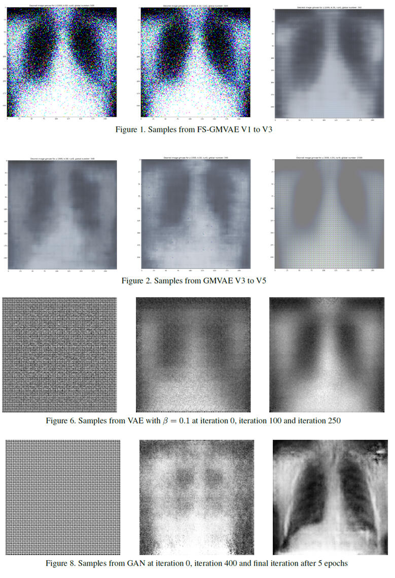
Why this Project?: At the time, generative modelling for creating synthetic chest X-rays was taking a boom, ever since GAN research has become much more complex, the invention of the latent diffusion models, and there were pretty good VAE model research (although their code was not public). Therefore, this group project focused into analyzing between VAE, GMVAE, and a Least Squares GAN to see which one produced the best images.
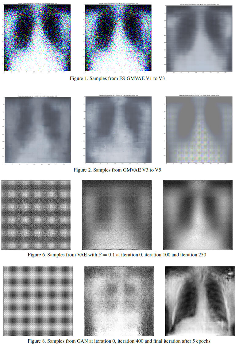
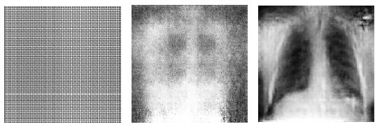
Results? The following images showcase the GAN, GMVAE, and VAE generated images. We can see how the least squared GANs seemed to have way better images, compared to GMVAE and VAE.


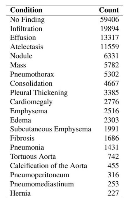
DatasetOur dataset consists of the NIH Chest X-rays images from 2018 to 2023. It contains different radiology images from 14 different chest X-rays conditions from posterior Anterior (PA), Anterior Posterior (AP), and lateral Projections (LAT) angles. The following are the amount of images per condition:
Data Preprocessing:
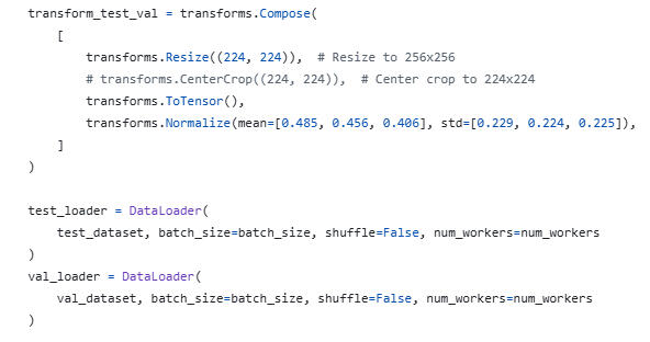
For the data preprocessing of each of the models, we used the same resizing and normalization methods in order to keep consistent inputs. There were some experiments that involved using histogram equalization as a different pre-processing step, althought results showcased that the images generated were kind of blueish at the end. Therefore, we preferred the normal gray scaliing
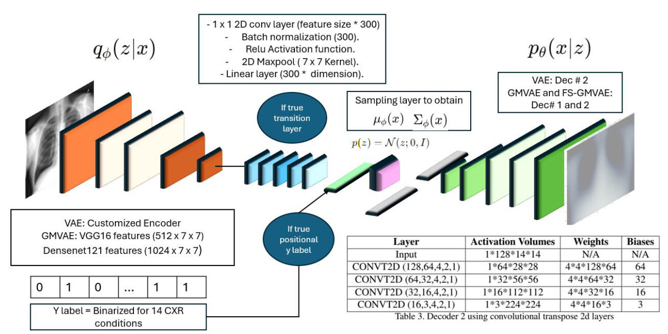
Model Architecture: GMVAEBuilding on my previous project in CS236, we replicated prior research on generating chest X-ray images using a Gaussian Mixture Variational Autoencoder (GMVAE). Our key improvement was refining the decoder architecture by incorporating transposed 2D convolution layers, which helped preserve spatial features and improve reconstruction quality. However, despite extensive experimentation and research (with more planned in the future), the latent space remained linear for the mean and variance distributions of the Gaussian mixture model.
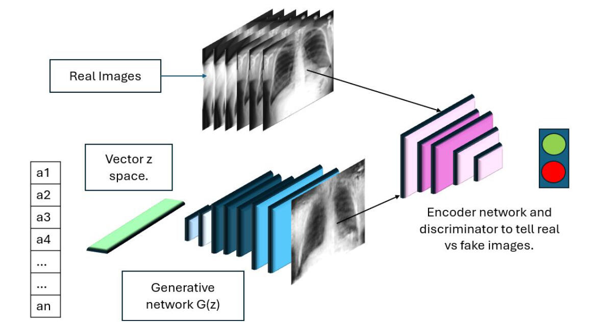
Model Architecture Least Squares GANWe chose to use a least squares GAN, since it has been found empirically with this dataset to be more stable for generation than normal GAN.

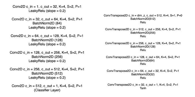
The purpose of it is to have two optimization techniques. While one conglomerate of neural networks act as a generator to generate synthetic images from real data, the discriminator would do its best to classify which ones are real and which ones are synthetic. The following diagrams showcase a diagram presentation of it; as well as which architectures we used for creating the GANs.
Conclusions and DiscussionAfter finishing this project, we found a couple of insights:
Using a better decoder with convolutional 2D transpose layers for the GMVAE and FS-GMVAE, didn't quite improve the image quality.
Truly, from previous research of CS236 project, I see that the Z-space used is too compressed to capture the complex anatomical structures.
Considesing Convolutional GMVAE with a more complex Z-space.
Regardless, using a convolutional GAN approach; we can see genuinely much better results than our current VAE approaches.
In the future, much more complex GAN architectures should be investigated as well.
If you want to learn more about the project, below are the links to the specific code sections that break the code, step by step.🖱️
CS231N: Specific Github Project Links to understand code🖥️
Least Squared GAN Codes:
- Project Code link: Discriminative or Generative Classifier for GAN
- Project Code link: Helper functions for GAN or VAE
- Project Code link: Least Squared GAN Code
VAE Codes:
GMVAE codes:
- Project Code link: CXR14 Python Download Code
- Project Code link: CXR14 PyTorch Dataset Reader.
- Project Code link: CXR14 Class Dataframe Reader
- Project Code link: Preprocessing and VAEs tools
- Project Code link: Training function Different VAEs.
- Project Code link: GMVAE Model:
- Project Code link: FS-GMVAE Model
- Project Code link: GMVAE Model
Emotion Segmentation using Bi-directional LSTMS and BERT Embeddings
Project Links below
Date: March 9th, 2024
Group Members:
Hannah Levin
Samir Agarwala
Juan Pablo Triana Martinez
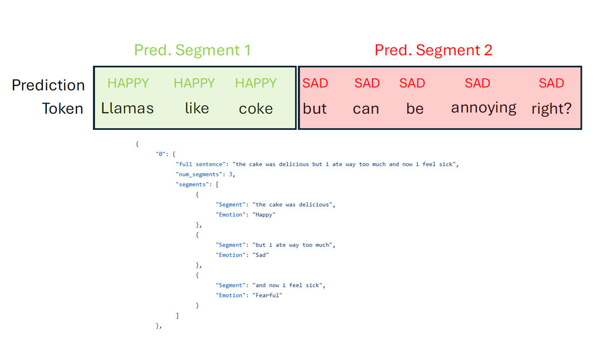
Why this project? At the time, research on emotion segmentation was a bit limited. Every effort was made to classify binary sentiment analysis, and research regarding emotion classification was done per sentence. However, no relevant research was found on a token of emotion per segment in a sentence. We know human language is complicated enough to contain multiple emotions in one sentence; therefore, our group project was developing an Emotion segmentation Deep Learning model using LLMs for data generation and Bi-directional LSTM Models.
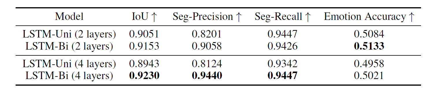
Results? By assesing segmentation quality using intersection over union between grouth truth segments and predicted segments, after removing punctuations and spaces, and emotion quality using accuracy between predicted segment emotion and ground truth segment emotion, we found our model to be superior to the baselines.
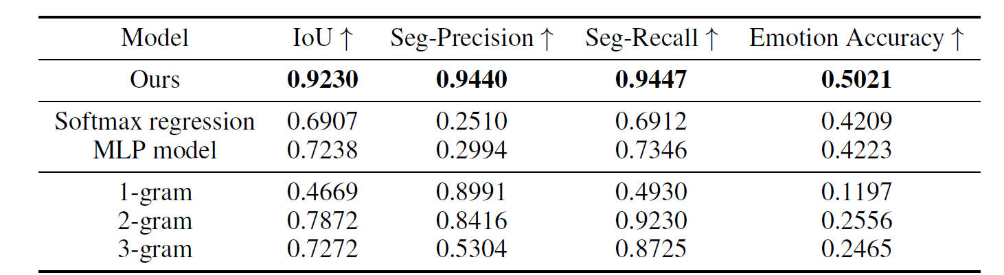
What was our model? We used Bi-directional LSTMS! The following image showcases different quantitative results for different configurations of LSTMs (Unidirectional, Bidirectional, 2 layers, or 4 layers)
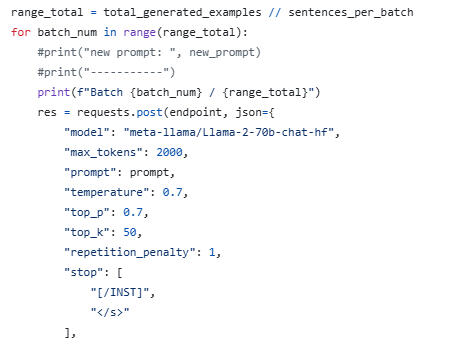
Dataset Generation: We opted for using Together API and a LLM to generate our data. We realized there were not a dataset that divided sentences into segments, annotated with their corresponding emotion. Therefore, we started testing different LLMs (Alpaca, Qwen1.5-72B-Chat, Llama-2-70B-Model). We chose LLama-2-70B due to:
Consistent Formatting (Respected the passed prompt examples).
Consistent emotions (Didnt create new emotions out of the blue).
Consistent generation of diverse examples when using iterative-batch approach (replace examples in the prompt from a previous batch).

Above was the prompt used to generate our dataset, and below are the parameters used for the LLM model.
Dataset Post-Processing: Althought we had 50,000 Examples created of different segments (1, 2, and 3). We still had to post-process it in order to retrieve proper examples. Specially, we found that:
There were repeated sentences, we had to discard the duplicates
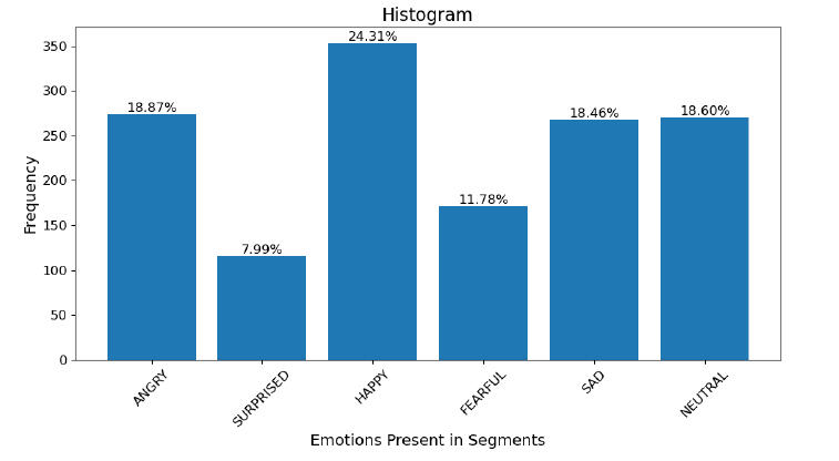
There was a lot of emotion imbalance across segments, we had to equalize the emotion distribution across examples.
After equalizing emotions, it was necessary to merge all different files into a proper format for analysis.
Because of this, we come up with:
Data Merging: A script that processes and combines multiple raw data files generated from an LLM, each corresponding to different segments, into a single consolidated file for an intermediate step.
Filtering Unique Entries: A script that removes unique entries from the merged dataset to retain only recurring data points for further analysis.
Balancing Emotional Distributions: A script that categorizes examples based on the number of segments, then balances the distribution of emotions by ensuring a minimum number of examples per emotion. For simplicity, sentences expressing multiple emotions are treated as independent events.
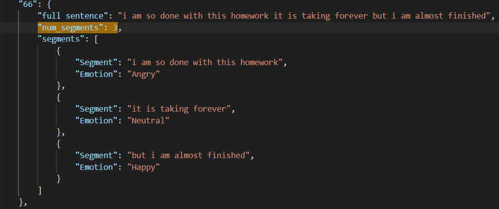
The final dataset contained 3,907 sentences (1, 2, and 3 segments). We split it into 75% training, 5% validation, and 20% test. The test set included 783 full sentences with 1,428 segments: 97 three-segment, 451 two-segment, and 235 one-segment.The following contains the emotion distribution , and one example, for sentences containing 1 segment.
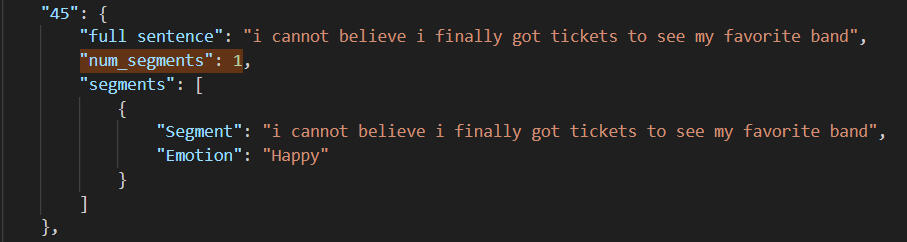
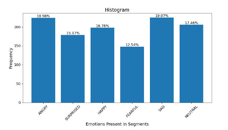
The following contains the emotion distribution, and one example, for sentences containing 2 segments.
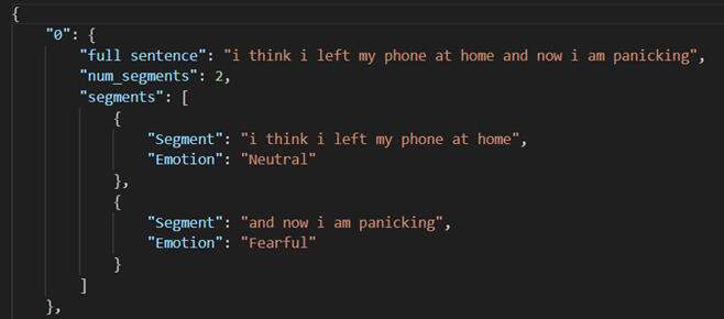
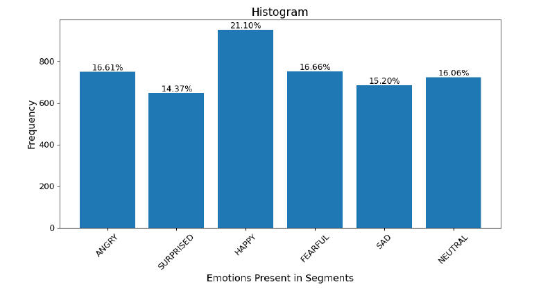
The following contains the emotion distribution, and one example, for sentences containing 3 segments.
Model Achitecture: Our model architecture consists of three main components: a frozen BERT tokenizer, a pretrained transformer BERT frozen sentence encoder, and the last layer consists of the models we are gonna analyze, these were:
N-gram models: Sentences were split into n equal segments, BERT encodings were computed, and emotions were assigned via cosine similarity (No training required).
Neural Network models: BERT encodings per word token were used for emotion prediction, testing a softmax model and an MLP.
LSTM models: Word tokens and embeddings were processed by different LSTM models to predict emotions.
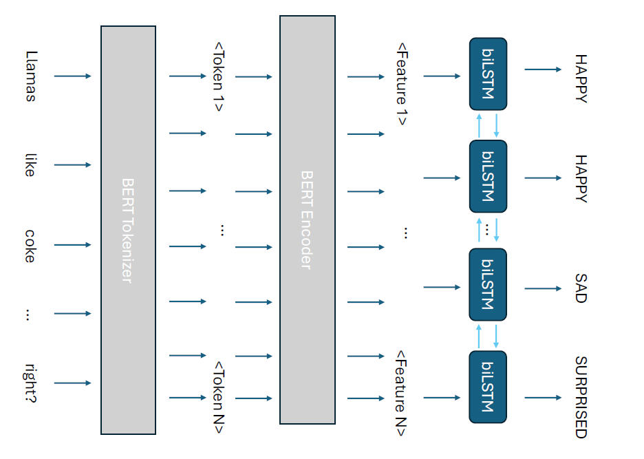
For neural networks and LSTMs, the predicted outputs were emotions per token. These were compared to the ground truth to assess segmentation quality and emotion classification accuracy.

Qualitative Results: Looking at a couple of examples showcased below: We can see that the Bidirectional-LSTM model has times where it nails it! But other times were is partly correct, and completely wrong.
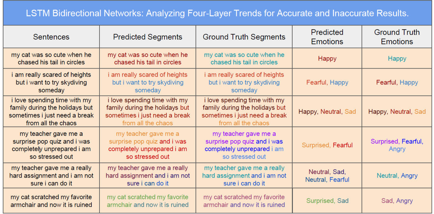
In the last three rows, we observed that while the model sometimes captured the intended emotions, it occasionally overpredicted or misclassified them.Interestingly, these errors were more aligned with negative emotions. Upon reviewing misclassified examples, we found that alternative emotional labels were also plausible from a human perspective.This suggests that incorporating broader context could enhance emotion prediction. In the future, we aim to explore transformer-based models to assess whether they better capture contextual dependencies.If you want to learn more about the project, below are the links to the specific code sections that break the code, step by step.🖱️
CS224N: Specific Github Project Links to understand code🖥️
- Project Code link: Llama-2-70-B Generation Code
- Project Code link: Merge LLM files
- Project Code link: Post-Processing Generated Sentences
- Project Code link: Equalizing Emotions in Sentence Segments
- Project Code link: Torch Dataset using BERT Tokenizer and Embeddings
- Project Code link: Utils for train, inference, and validation.
- Project Code link: LSTM model architecture
- Project Code link: Baseline MLP model
- Project Code link: Baseline n-gram model
- Project Code link: Baseline regression softmax model
- Project Code link: Training code for deep learning models.
GENERATE CHEST X-RAYS USING GMVAE AND DIFFERENT LOSSES (MSE AND BCE)
Project Links below
Date: December 15th, 2023
Group Members:
Kuniaki Iwanami
Juan Pablo Triana Martinez
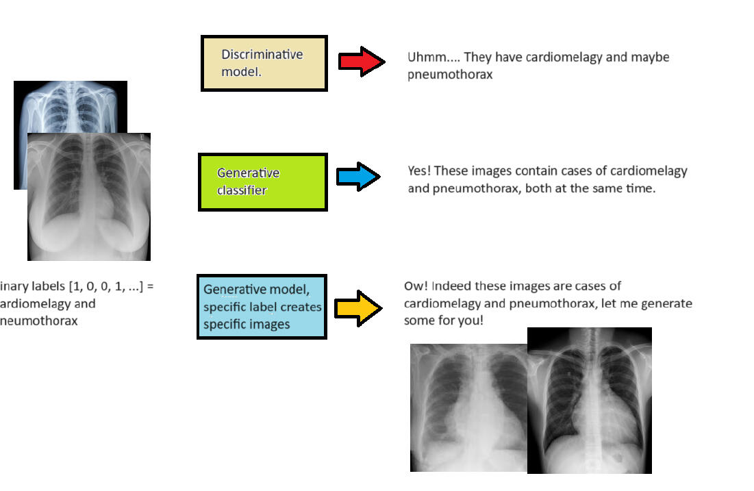
Why this Project? At the time, there was a lot of research being proposed for multi-classificaiton of different lung pathologies in Chest X-rays images using create generative classifiers, instead of discriminative classifiers (VggNet16, DenseNet16, AlexNet16). Therefore, our group wanted to see the possibility of using this comprised generative feature space (freezing weight parameters of encoder side), but for the task of image generation! Especially, how feasible it was to use a simple decoder, and simple probabilistic representations (Gaussian) to recreate the complex structures of the human body.
Results? We used Variational Autoencoders for this project. We knew we needed the feature space to be way more complex than a VAE, so we used a Gaussian mixture VAE to start with BCE loss, MSE loss, and a combination of both! We used a z space of length = 1280, K-Gaussians = 500, and 2000 Iterations. The results are shown below:
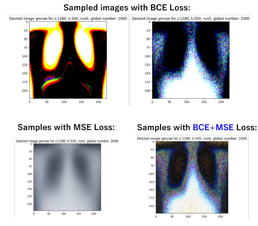
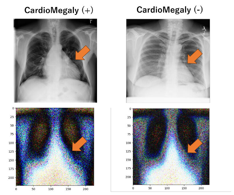
Althought the images were not that great quality, we saw with our research three possibilities to improve this was: Unfroze the encoder weights to allow VAE proper training (we couldn't do it at the time due to computation resources), a much better decoder (you will see the architecture later), and a much better Z-space representation for our generative model representation. NEVERTHERLESS we did an innovative approach; we concatenated a positional embedding vector of size 14, [of ones and zeroes], to train a FS-GMVAE. This allowed us to retrieve specific images in inference for specific medical conditions.
Variational Auto-Encoder Math
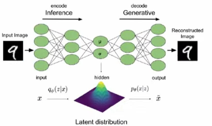
Before we continue with this project. I would like to show a bit of mathematical theory regarding Variational Auto-Encoders. Specifically to illustrate how these work, and how the gaussian mixed-mixture VAE model Idea came to be when we were performing this research project.By using probabilistic inference, and Bayesian Statistics, VAEs would model the desired data distribution through a latent space, and explicitly calculate the probability density of the data by integrating over the latent space.Therefore, we can use a simple P(z) space (a gaussian probability distribution), and smaller components P(x|z) (Gaussian Component) to represent really complex distributions, as shown below:

The VAE components are:
Encoder: Extract features from higher dimension space to lower dimension space.
Latent Space: We normally use neural networks here to represent it. For a mixed Gaussian, this would be the mean and variance. This is passed then to a sampling layer to feed to the decoder to reconstruct the image.
Decoder: It takes sampled z-vectors from the z-distribution feature space and feeds them to reconstruct an image.
The primary ojective of the VAE is Maximum likelihood estimation. This is done via Monte Carlo to sample in an intelligent way our z space, using an ideal probability distribution that for now we will call q(z)


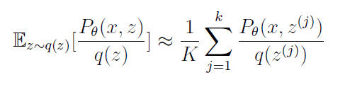
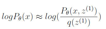
Wait there is a caveat here. Lets assume k = 1. When we apply the log function to our new Monte Carlo Representation of P(x), we get:
Jensen Inequality
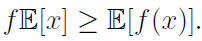
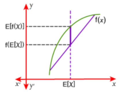
In a concave function. The upper limit is defined as the Expected value of f(x) , while the lower limit is the the function of expected of x. Why do we need this?. Well, this means that our limits for the VAE Formulation would be:
Upper Limit
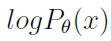
Lower Limit
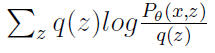
Continuing the derivation, we see the following:
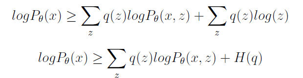
The lower bound would be equal to the upper bound only when the first image becomes true. Giving rise to the second Image (KL divergence ).
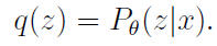


There is a problem. Tracking p(z|x) with theta parameters becomes untrackable, we then perform the following to optimize to a much easier distribution with set of parameters alpha.

With this likelihood based on parameters alpha and theta, we apply a parametrization and amortization (this is a bit too advanced to see here lol). So we can do the following derivation using expectations, summations, and log rules.
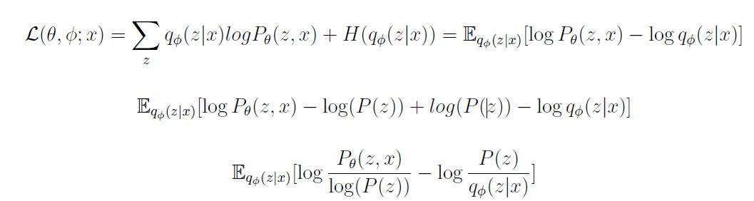
FINALLY WE GET THIS This is even represented with the graphical diagram below. This is how we can obtain a VAE using much simpler statistical probabilities, to represent much complex data:

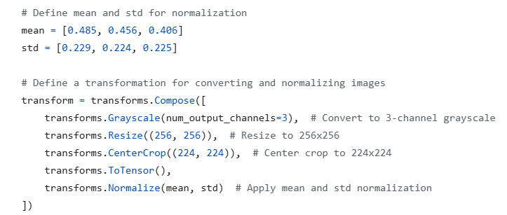
Data Preprocessing: Before we passed the Chest X-ray images, we had to preprocess them enough since we chose to use VGG16 feature space as our encoder. Their architecture accept 3x224x224 inputs. We had to do the follow:
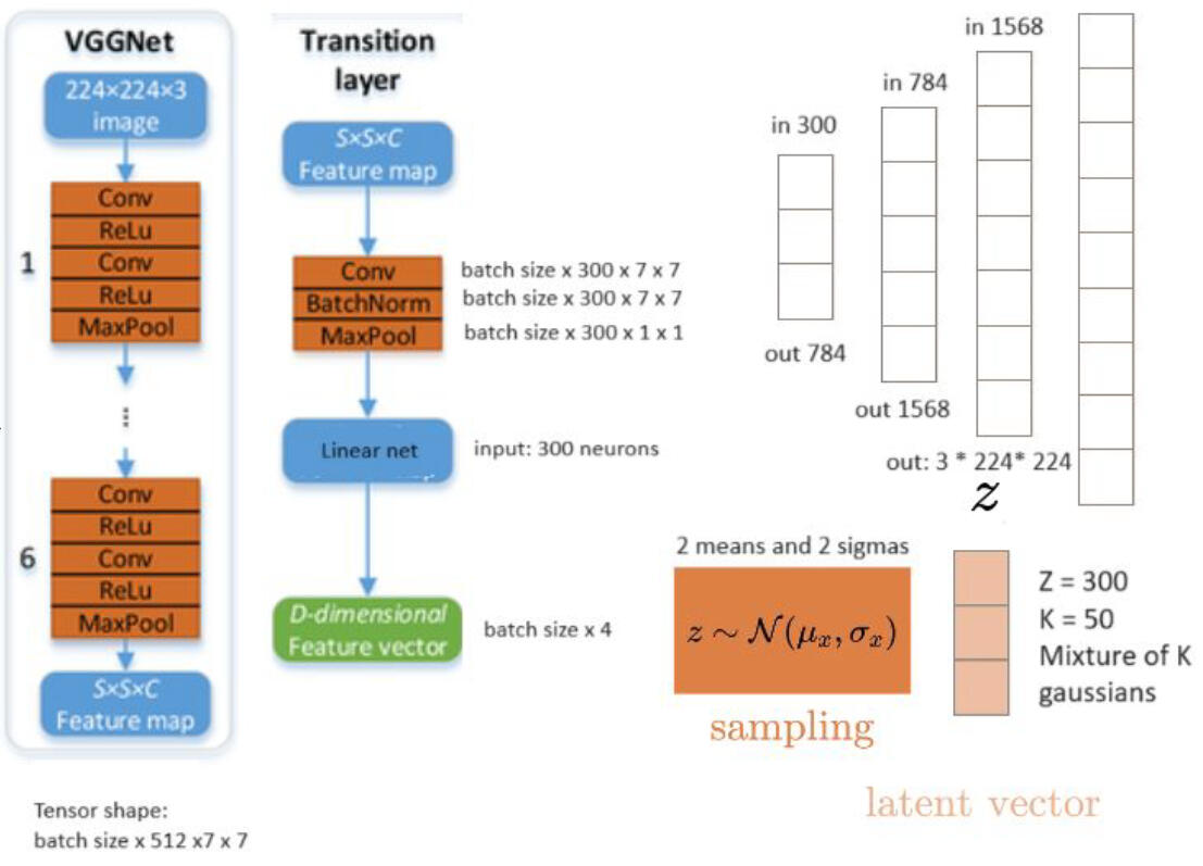
Model Architecture: The following image illustrate the model architecture we used in order to create our GMVAE and FS-GMVAE
Overall, this was a good project to introduce us to the VAE model and the different kinds. We also saw how to set up this generative approach with medical image data.We got pretty good insights on what could be done in the future to improve the model, such as: Allow for the encoder to train in the likelihood function, Gaussian mixtures seems that its limited until a certain point; maybe a convolutional VAE for a spatial z space, much more computing power, and a better decoder than just simple layers.If you want to learn more about the project, below are the links to the specific code sections that break the code, step by step.🖱️
CS236: Specific Github Project Links to understand code🖥️
- Dataset Link | Chest X-ray-14 | year 2018-2023
- Project Code link: CXR14 Python Download Code
- Project Code link: CXR14 PyTorch Dataset Reader.
- Project Code link: CXR14 Class Dataframe Reader
- Project Code link: GMVAEs and FS-VAEs tools
- Project Code link: Training function Different VAEs.
- Project Code link: GMVAE Model:
- Project Code link: FS-GMVAE Model
- Project Code link: Run FS-GMVAE Model
- Project Code link: Run GMVAE Model